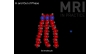
This is an animation that supports Figure 6.5, and the explanation of this diagram in the book. It shows what happens in a spin echo pulse sequence with three slices. Each slice has its own area of k-space, and is represented by a chest of drawers. The application of the RF excitation pulse and the slice select gradient picks chest of drawers or k-space area or slice 1. The phase encoding gradient switches on next and the slope and the polarity of this gradient determines which drawer or k-space line will be used. In the animation, the slope and the polarity of the phase encoding gradient is such that the third drawer down in the chest of drawers is opened. The next occurrence in the sequence is the application of the 180° RF rephasing pulse, but ignore this for the time being - we'll get to it later in the chapter. The next thing that happens in the sequence is the frequency encoding gradient that is switched on as the echo occurs. The frequencies in the echo are sampled at this point, and the data points (or socks in the animation) are put into this drawer or line of k-space. When the frequency encoding gradient is switched off, this is equivalent to shutting the drawer. Next the 90° RF excitation pulse and slice select gradient are applied to slice 2. This selects chest of drawers or k-space area 2. The phase encoding gradient is switched on again, to the same slope and polarity as it was applied for chest of drawers 1. This therefore opens the same drawer in chest of drawers 2 as it did in chest of drawers 1. The frequency encoding gradient is then applied as the echo occurs in slice 2. Frequencies in the echo are sampled, and the data from them is laid out in the open draw in chest of drawers 2. Once the frequency encoding gradient is switched off, the drawer closes, and the RF excitation pulse and slice select gradient are applied to chest of drawers 3. The phase encoding gradient is applied again to the same slope and polarity as it was applied for chest of drawers 1 and 2. This therefore opens the third draw down in the chest of drawers 3. The frequency encoding gradient is switched on again, and the frequencies from the echo are collected and laid out in this drawer. Switching the frequency encoding gradient off closes the drawer for this chest of drawers. All this occurs in the TR period as shown in the animation. In the next TR period, the RF excitation pulse and slice select gradient are applied again to slice or chest of drawers 1, but the slope of the phase encoding gradient is changed to open a different drawer. The sequence is repeated, changing the slope of the phase gradient in every TR to fill a different drawer in each of the chest of drawers until all the drawers in every chest of drawers are filled with data.
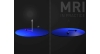 Animation 1.1 Rotating and Fixed Frame of Reference
09/05/2023
Animation 1.1 Rotating and Fixed Frame of Reference
09/05/2023
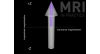
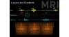
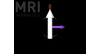 Animation 1.2 (NMV and Coil)
09/05/2023
Animation 1.2 (NMV and Coil)
09/05/2023
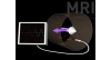 Animation 1.3 (NMV Coil and Oscilloscope)
09/05/2023
Animation 1.3 (NMV Coil and Oscilloscope)
09/05/2023
 Animation 2.1 (T1 vs T2)
09/05/2023
Animation 2.1 (T1 vs T2)
09/05/2023
 Animation 2.2 (Diffusion)
09/05/2023
Animation 2.2 (Diffusion)
09/05/2023
 Animation 3.1 (The 180° RF Pulse)
09/05/2023
Animation 3.1 (The 180° RF Pulse)
09/05/2023
 Animation 3.2 (The Larmor Grand Prix)
09/05/2023
Animation 3.2 (The Larmor Grand Prix)
09/05/2023
 Animation 3.3 Inversion Recovery
09/05/2023
Animation 3.3 Inversion Recovery
09/05/2023
 Animation 6.1 (Slices Chest of Drawers)
09/05/2023
Animation 6.1 (Slices Chest of Drawers)
09/05/2023
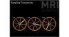 Animation 6.2. (Sampling Frequencies)
09/05/2023
Animation 6.2. (Sampling Frequencies)
09/05/2023
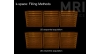 Animation 6.3 (Filling Methods)
09/05/2023
Animation 6.3 (Filling Methods)
09/05/2023
 Animation 8.1 (In and Out of Phase)
09/05/2023
Animation 8.1 (In and Out of Phase)
09/05/2023
 Animation 8.2 (Entry-slice Phenomenon)
09/05/2023
Animation 8.2 (Entry-slice Phenomenon)
09/05/2023
 Animation 8.3 Time of Flight
09/05/2023
Animation 8.3 Time of Flight
09/05/2023
 Animation 8.4 (Gradient Moment Nulling)
09/05/2023
Animation 8.4 (Gradient Moment Nulling)
09/05/2023
 Animation 9.1 (Closed and Open Systems)
09/05/2023
Animation 9.1 (Closed and Open Systems)
09/05/2023
 Animation 9.2 (Active Shielding)
09/05/2023
Animation 9.2 (Active Shielding)
09/05/2023
 Animation 9.3 (NMV Coil and Scanner Loop)
09/05/2023
Animation 9.3 (NMV Coil and Scanner Loop)
09/05/2023