Animation 6.2. (Sampling Frequencies)

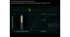
This is an animation that supports Figure 6.9. It demonstrates a good analogy that will help you understand the Nyquist theorem. Imagine there are three wheels turning in front of you, each turning at a different frequency. One wheel is rotating at a frequency of 1 Hz, another at a frequency of 2 Hz, and a third wheel at a frequency of 4 Hz. One of the spokes of the wheel is colored white so that you can appreciate the different frequencies more clearly. Imagine that you want to take photographs of these wheels turning using a camera that takes pictures at a frequency of the four photographs per second. In other words, it is taking photographs at a frequency of 4 Hz. The first wheel we are going to take pictures of is the 1 Hz wheel. The first photograph will be taken a quarter of a second after the wheel starts turning. The second photograph will be taken a quarter of a second after that, the third, quarter of a second after this, and the final photograph will be taken exactly one second after the wheel began to turn. You can see from the animation that the first photograph shows that the white spoke has moved through 90°. In the second photograph, it has moved another 90°, in the third photograph a further 90°, and in the final photograph, the white spoke has returned to its original position. Each photograph, therefore, shows the white spoke in a different positions. Let us compare these photographs with those of the 2 and 4 Hz wheels. You can see in the animation that the photographs taken after a quarter of a second show the white spoke moving through 90° on the 1 Hz wheel, 180° on the 2 Hz wheel, and a full 360° on the 4 Hz wheel. The second set of photographs show that the white spoke moves through a further 90° on the 1 Hz wheel, but on the 2 and 4 Hz wheels it has moved back to its starting position. Watch how the position of the white spoke changes in the third and fourth set of photographs for all three wheels.

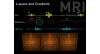
Now let us look at the set of photographs taken at each time frame for the 1 Hz wheel. You can see that the white spoke has a different position on every photograph. It is therefore easy to see that the wheel turned while the photographs were being taken. The set of photographs from the 2 Hz wheel shows that the white spoke only has two different positions. Although we can tell that the wheel was turning while the photographs were being taken, we do not necessarily know which direction the wheel was turning. Now look at the photographs taken of the 4 Hz wheel. The white spoke is at the same position on each photograph, and we are, therefore, unable to tell whether that wheel was moving or not. This is because we have taken pictures at the same frequency (4 Hz) as the wheel was turning. In other words, we have not taken pictures quickly enough to know whether the 4 Hz wheel is turning or not.

The Nyquist theorem explains this concept when converting an analogue signal (a waveform) into a series of digitized data points. The Nyquist theorem says that in order to know what frequency a waveform has, we must sample or measure it at a frequency that is at least twice as high as the waveforms' frequency. In our photograph and wheel analogy, therefore, we are sampling the wheels at a frequency of 4 Hz and therefore, we have enough information about the 1 and 2 Hz wheels to know what their frequencies are. However, we do not have enough information about the 4 Hz wheel because we have not sampled it fast enough - we have only sampled it at exactly the same frequency, not at twice this frequency. In MRI, as we have a modulation of several frequencies to sample, the Nyquist theorem is slightly modified - it states that we must sample at least twice as high as the highest frequency present in the modulation in order to sample it often enough.